Linear Regression in Business Statistics

The task of bringing out linear relationship consists of developing methods of fitting a straight line, or a regression line as is often called, to the data on two variables.

The line of Regression is the graphical or relationship representation of the best estimate of one variable for any given value of the other variable. The nomenclature of the line depends on the independent and dependent variables. If X and Y are two variables of which relationship is to be indicated, a line that gives best estimate of Y for any value of X, it is called Regression line of Y on X. If the dependent variable changes to X, then best estimate of X by any value of Y is called Regression line of X on Y.

• REGRESSION LINE OF Y ON X

 For purposes of illustration as to how a straight line relationship is obtained, consider the sample paired data on sales of each of the N = 5 months of a year and the marketing expenditure incurred in each month, as shown in Table 5-1

Let Y, the sales, be the dependent variable and X, the marketing expenditure, the independent variable. We note that for each value of independent variable X, there is a specific value of the dependent variable Y, so that each value of X and Y can be seen as paired observations.

• Scatter Diagram

 Before obtaining a straight-line relationship, it is necessary to discover whether the relationship between the two variables is linear, that is, the one which is best explained by a straight line. A good way of doing this is to plot the data on X and Y on a graph so as to yield a scatter diagram, as may be seen in Figure 5-1. A careful reading of the scatter diagram reveals that:

• the overall tendency of the points is to move upward, so the relationship is positive
• the general course of movement of the various points on the diagram can be best explained by a straight line
• there is a high degree of correlation between the variables, as the points are very close to each other

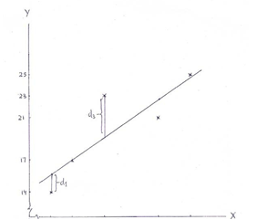
Figure 5-1    Scatter Diagram with Line of Best Fit

Fitting a Straight Line on the Scatter Diagram

If the movement of various points on the scatter diagram is best described by a straight line, the next step is to fit a straight line on the scatter diagram. It has to be so fitted that on the whole it lies as close as possible to every point on the scatter diagram. The necessary requirement for meeting this condition being that the sum of the squares of the vertical deviations of the observed Y values from the straight line is minimum.

As shown in Figure 5-1, if d_l, d₂,..., d_N are the vertical deviations' of observed Y values from the straight line, fitting a straight line requires that

is the minimum. The deviations d_j have to be squared to avoid negative deviations canceling out the positive deviations. Since a straight line so fitted best approximates all the points on the scatter diagram, it is better known as the best approximating line or the line of best fit. A line of best fit can be fitted by means of:

2. Free hand drawing method, and
3. Least square method

1. Free Hand Drawing:

Free hand drawing is the simplest method of fitting a straight line. After a careful inspection of the movement and spread of various points on the scatter diagram, a straight line is drawn through these points by using a transparent ruler such that on the whole it is closest to every point. A straight line so drawn is particularly useful when future approximations of the dependent variable are promptly required.

Whereas the use of free hand drawing may yield a line nearest to the line of best fit, the major drawback is that the slope of the line so drawn varies from person to person because of the influence of subjectivity. Consequently, the values of the dependent variable estimated on the basis of such a line may not be as accurate and precise as those based on the line of best fit.

2. Least Square Method:

The least square method of fitting a line of best fit requires minimizing the sum of the squares of vertical deviations of each observed Y value from the fitted line. These deviations, such as d₁ and d₃, are shown in Figure 5-1 and are given by Y - Y_c, where Y is the observed value and Y_c the corresponding computed value given by the fitted line Yc = a + bX i for the i^th value of X.

The straight line relationship in Eq.(5.1), is stated in terms of two constants a and b

• The constant a is the Y-intercept; it indicates the height on the vertical axis from where the straight line originates, representing the value of Y when X is zero.
• Constant b is a measure of the slope of the straight line; it shows the absolute change in Y for a unit change in X. As the slope may be positive or negative, it indicates the nature of relationship between Y and X. Accordingly, b is also known as the regression coefficient of Y on X.

Since a straight line is completely defined by its intercept a and slope b, the task of fitting the same reduces only to the computation of the values of these two constants. Once these two values are known, the computed Y_c values against each value of X can be easily obtained by substituting X values in the linear equation.

In the method of least squares the values of a and b are obtained by solving simultaneously the following pair of normal equations

Note: Eq. (5.3) is obtained simply by dividing both sides of the first of Eqs. (5.2) by N and Eq.(5.4) is obtained by substituting (Y - b X ) in place of a in the second of Eqs. (5.2)

Instead of directly computing b, we may first compute value of a as

            Y                   X                     XY                                X²                               Y²

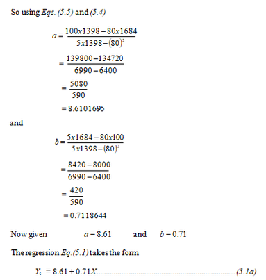
Figure: Regression Line of Y on X

Then, to fit the line of best fit on the scatter diagram, only two computed Y_c values are needed. These can be easily obtained by substituting any two values of X in Eq. (5.1a). When these are plotted on the diagram against their corresponding values of X, we get two points, by joining which (by means of a straight line) gives us the required line of best fit, as shown in Figure 5-2

Some Important Relationships

Predicting an Estimate and its Preciseness

The main objective of regression analysis is to know the nature of relationship between two variables and to use it for predicting the most likely value of the dependent variable corresponding to a given, known value of the independent variable. This can be done by substituting in Eq.(5.1a) any known value of X corresponding to which the most likely estimate of Y is to be found.

For example, the estimate of Y (i.e. Y_c), corresponding to X = 15 is

Y_c = 8.61 + 0.71(15) = 8.61 + 10.65 = 19.26

It may be appreciated that an estimate of Y derived from a regression equation will not be exactly the same as the Y value which may actually be observed. The difference between estimated Y_c values and the corresponding observed Y values will depend on the extent of scatter of various points around the line of best fit.

The closer the various paired sample points (Y, X) clustered around the line of best fit, the smaller the difference between the estimated Y_c and observed Y values, and vice-versa. On the whole, the lesser the scatter of the various points around, and the lesser the vertical distance by which these deviate from the line of best fit, the more likely it is that an estimated Y_c value is close to the corresponding observed Y value.

The estimated Y_c values will coincide the observed Y values only when all the points on the scatter diagram fall in a straight line. If this were to be so, the sales for a given marketing expenditure could have been estimated with l00 percent accuracy. But such a situation is too rare to obtain. Since some of the points must lie above and some below the straight line, perfect prediction is practically non-existent in the case of most business and economic situations.

This means that the estimated values of one variable based on the known values of the other variable are always bound to differ. The smaller the difference, the greater the precision of the estimate, and vice-versa. Accordingly, the preciseness of an estimate can be obtained only through a measure of the magnitude of error in the estimates, called the error of estimate.

Error of Estimate

A measure of the error of estimate is given by the standard error of estimate of Y on X, denoted as S_yx and defined as

S_yx measures the average absolute amount by which observed Y values depart from the corresponding computed Y_c values.

Computation of S_yx becomes little cumbersome where the number of observations N is large. In such cases S_yx may be computed directly by using the equation:

Interpretations of S_yx

A careful observation of how the standard error of estimate is computed reveals the following:

1. S_yx is a concept statistically parallel to the standard deviation S_y . The only difference between the two being that the standard deviation measures the dispersion around the mean; the standard error of estimate measures the dispersion around the regression Similar to the property of arithmetic mean, the sum of the deviations of different Y values from their corresponding estimated Y_c values is equal to zero. That is å( Y_i - Y ) = å ( Y_i - Y_c) = 0 where i = 1, 2, ..., N.

2. S_yx tells us the amount by which the estimated Y_c values will, on an average, deviate from the observed Y Hence it is an estimate of the average amount of error in the estimated Y_c values. The actual error (the residual of Y and Y_c) may, however, be smaller or larger than the average error. Theoretically, these errors follow a normal distribution. Thus, assuming that n ≥ 30, Y_c ± 1.S_yx means that 68.27% of the estimates based on the regression equation will be within 1.S_yx Similarly, Y_c ± 2.S_yx means that 95.45% of the estimates will fall within 2.S_yx

Further, for the estimated value of sales against marketing expenditure of Rs 15 thousand being Rs 19.26 lac, one may like to know how good this estimate is. Since S_yx is estimated to be Rs 2.16 lac, it means there are about 68 chances (68.27) out of 100 that this estimate is in error by not more than Rs 2.16 lac above or below Rs

19.26 lac. That is, there are 68% chances that actual sales would fall between (19.26 - 2.16) = Rs 17.10 lac and (19.26 + 2.16) = Rs 21.42 lac.

3. Since S_yx measures the closeness of the observed Y values and the estimated Y_c values, it also serves as a measure of the reliability of the estimate. Greater the closeness between the observed and estimated values of Y, the lesser the error and, consequently, the more reliable the estimate. And vice-versa.
4. Standard error of estimate S_yx can also be seen as a measure of correlation insofar as it expresses the degree of closeness of scatter of observed Y values about the regression The closer the observed Y values scattered around the regression line, the higher the correlation between the two variables.

A major difficulty in using S_yx as a measure of correlation is that it is expressed in the same units of measurement as the data on the dependent variable. This creates problems in situations requiring comparison of two or more sets of data in terms of correlation. It is mainly due to this limitation that the standard error of estimate is not generally used as a measure of correlation. However, it does serve as the basis of evolving the coefficient of determination, denoted as r², which provides an alternate method of obtaining a measure of correlation.

REGRESSION LINE OF X ON Y

A major difficulty in using S_yx as a measure of correlation is that it is expressed in the same units of measurement as the data on the dependent variable. This creates problems in situations requiring comparison of two or more sets of data in terms of correlation. It is mainly due to this limitation that the standard error of estimate is not generally used as a measure of correlation. However, it does serve as the basis of evolving the coefficient of determination, denoted as r², which provides an alternate method of obtaining a measure of correlation.

REGRESSION LINE OF X ON Y

So far we have considered the regression of Y on X, in the sense that Y was in the role of dependent and X in the role of an independent variable. In their reverse position, such that X is now the dependent and Y the independent variable, we fit a line of regression of X on Y. The regression equation in this case will be

For example, if we want to estimate the marketing expenditure to achieve a sale target of Rs 40 lac, we have to obtain regression line of X on Y i. e.

Now given that a’= -5.00 and b’=1.05, Regression equation (5.13) takes the form

X_c = -5.00 +1.05Y

So when Y = 40(Rs lac), the corresponding X value is X_c = -5.00+1.05x40 = -5 + 42 = 37

That is to achieve a sale target of Rs 40 lac, there is a need to spend Rs 37 thousand on marketing.