- Optical signals of different wavelength (1300-1600 nm) can propagate without interfering with each other. The scheme of combining a number of wavelengths over a single fiber is called wavelength division multiplexing (WDM).
- Each input is generated by a separate optical source with a unique wavelength. An optical multiplexer couples light from individual sources to the transmitting fiber. At the receiving station, an optical demultiplexer is required to separate the different carriers before photodetection of individual Fig. 7.1.1 shows simple SDM scheme.
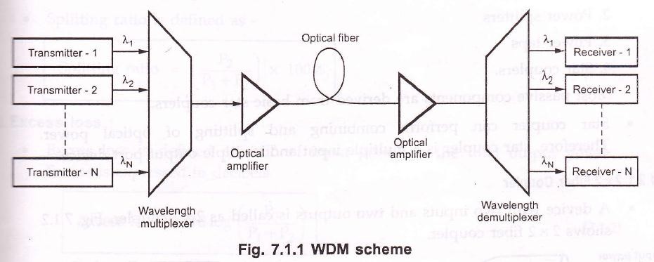
- To prevent spurious signals to enter into receiving channel, the demultiplexer must have narrow spectral operation with sharp wavelength cut-offs. The acceptable limit of crosstalk is – 30 dB.
Features of WDM
- Important advantages or features of WDM are as mentioned below –
- Capacity upgrade : Since each wavelength supports independent data rate in
- Transparency : WDM can carry fast asynchronous, slow synchronous, synchronous analog and digital data.
- Wavelength routing : Link capacity and flexibility can be increased by using multiple
- Wavelength switching : WDM can add or drop multiplexers, cross connects and wavelength
Passive Components
- For implementing WDM various passive and active components are required to combine, distribute, isolate and to amplify optical power at different wavelength.
- Passive components are mainly used to split or combine optical These components operates in optical domains. Passive components don’t need external control for their operation. Passive components are fabricated by using optical fibers by planar optical waveguides. Commonly required passive components are –
- N x N couplers
- Power splitters
- Power taps
- Star
Most passive components are derived from basic stat couplers.
- Stat coupler can person combining and splitting of optical power. Therefore, star coupler is a multiple input and multiple output port device.
2 x 2 Fiber Coupler
- A device with two inputs and tow outputs is called as 2 x 2 coupler. Fig. 7.1.2 shows 2 x2 fiber
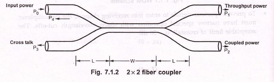
- Fused biconically tapered technique is used to fabricate multiport couplers.
- The input and output port has long tapered section of length ‘L’.
- The tapered section gradually reduced and fused together to form coupling region of length ‘W’.
- Input optical power : P0. Throughtput power : P1. Coupled power : P2. Cross talk : P3.
Power due to refelction : P4.
- The gradual tapered section determines the reflection of optical power to the input port, hence the device is called as directional coupler.
- The optical power coupled from on fiber to other is dependent on-
- Axial length of coupling region where the fields from fiber
- Radius of fiber in coupling
- The difference in radii of two fibers in coupling
Performance Parameters of Optical Coupler
- Splitting ratio / coupling ratio
- Splitting ratio is defined as –
 … (7.1.1)
2. Excess loss:
- Excess loss is defined as ratio of input power to the total output power. Excess is expressed in decibels.
![]() … (7.1.2)
… (7.1.2)
3. Insertion loss:
- Insertion loss refers to the loss for a particular port to port path. For path from input port I to output port j.
![]() …(7.1.3)
…(7.1.3)
4. Cross talk :
- Cross talk is a measure of degree of isolation between input port and power scattered or reflected back to other input port.

Example 7.1.1 : For a 2 x 2 fiber coupler, input power is 200 µW, throughput power is 90 µW, coupled power is 85 µW and cross talk power is 6.3 µW. Compute the performance parameters of the fiber coupler.
Solution : P0 = 200 µW
P1 = 90 µW P2 = 85 µW P3 = 6.3 µW
i)
![]()
![]()
Coupling ratio = 48.75 % … Ans.
ii)
![]()
![]() … Ans.
… Ans.
iii)
![]()
(For port 0 to port 1)
![]()
= 3.46 dB … Ans.
![]()
(For port 0 to port 2)
![]()

= 3.71 dB … Ans.
iv)

![]()
= -45 dB … Ans.
Star Coupler
- Star coupler is mainly used for combining optical powers from N-inputs and divide them equally at M-output ports.
- The fiber fusion technique is popularly used for producing N x N star coupler. Fig. 7.1.3 shows a 4 x 4 fused star coupler.

- The optical power put into any port on one side of coupler is equally divided among the output Ports on same side of coupler are isolated from each other.
- Total loss in star coupler is constituted by splitting loss and excess loss.
![]() … (7.1.4)
… (7.1.4)
![]() … (7.1.5)
… (7.1.5)
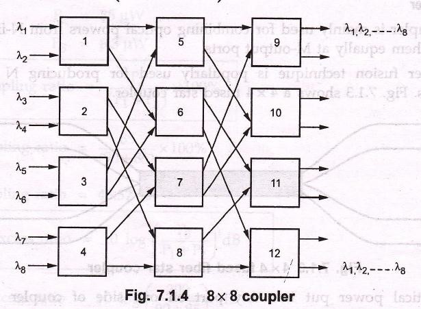
8 x 8 Star Coupler
- An 8 x 8 star coupler can be formed by interconnecting 2 x 2 couplers. It requires twelve 2 x 2 couplers.
- Excess loss in dB is given as –
![]() … (7.1.6)
… (7.1.6)
where FT is fraction of power traversing each coupler element.
Splitting loss = 10 log N
Total loss = Splitting loss + Excess loss
= 10 (1 – 3.32 log FT)log N
Wavelength converter
- Optical wavelength converter is a device that converts the signal wavelength to new wavelength without entering the electrical domain.
- In optical networks, this is necessary to keep all incoming and outgoing signals should have unique wavelength.
- Two types of wavelength converters are mostly used :
- Optical gating wavelength converter
- Wave mixing wavelength converter
Passive Linear Bus Performance
- For evaluating the performance of linear bus, all the points of power loss are
- The ratio (A0) of received power P(x) to transmitted power P(0) is
![]() … (7.9.1)
… (7.9.1)
where,
α is fiber attenuation (dB/km)
- Passive coupler in a linear bus is shown in 7.1.5 where losses encountered.

- The connecting loss is given by –
![]() … (7.1.10)
… (7.1.10)
where,
FC is fraction of optical power lost at each port of coupler.
- Tap loss is given by –
![]() … (7.1.11)
… (7.1.11)
where,
CT is fraction of optical power delivered to the port.
- The power removed at tap goes to the unused port hence lost from the The
throughput coupling loss is given by –
![]()
![]() … (7.1.12)
… (7.1.12)
- The intrinsic transmission loss is given as –
![]() … (7.1.13)
… (7.1.13)
where, Fi is fraction of power lost in the coupler.
- The fiber attenuation between two stations, assuming stations are uniformly separated by distance L is given by –
![]() … (7.1.14)
… (7.1.14)
Power budget
- For power budget analysis, fractional power losses in each link element is The power budget analysis can be studied for two different situations.
- Nearest-neighbour power budget
- Larget-distance power
1. Nearest-neighbour power budget
- Smallest distance power transmission occurs between the adjacent stations g. between station 1 and station 2.
- If P0 is optical power launched at station 1 and P1,2 is optical power detected at station
- Fractional power losses occurs at following
- Two tap points, one for each station.
- Four connecting points, two for each
- Two couplers, one for each
- Expression for loss between station 1 and station 2 can be written as –
![]() … (7.1.15)
… (7.1.15)
2. Larget distance power budget
- Largest distance power transmission occurs between station 1 and station
- The losses increases linearly with number of stations N.
- Fractional losses are contributed by following
- Fiber attenuation loss
- Connector loss
- Coupler throughput loss
- Intrinsic transmission loss
- Tao loss
- The expression for loss between station 1 and station N can be written as –
 … (7.1.16)
 … (7.1.17)
Example 7.1.3 : Prepare a power budget for a linear bus LAN having 10 stations. Following individual losses are measured.
Ltap = 10 dB Lthru = 0.9 dB
Li = 0.5 dB Lc = 1.0 dB
The stations are separated by distance = 500 m and fiber attenuation is 0.4 dB/km. Couple total loss in dBs.
Solution :
N = 10
L = 500 m = 0.5 km
α = 0.4 dB/km
![]()
= 10(0.4 x 0.5 + 2 x 1 + 0.9 + 0.5) – (0.4 x 0.5) – (2 x 0.9) + (2 x 10)
= 54 dB … Ans.
Star Network Performance
- If PS is the fiber coupler output power from source and P is the minimum optical power required by receiver to achieve specified BER.
- Then for link between two stations, the power balance equation is given by
PS-PR = Lexcess + α (2L) + 2Lc + Lsplit
where,
Lexcess is excess loss for star coupler (Refer equation 7.1.13),
Lsplit is splitting loss for star coupler (Refer equation 7.1.12), α is fiber attenuation,
L is distance from star coupler, Lc is connector loss.
- The losses in star network increases much slower as compared to passive liner bus. 7.1.6 shows total loss as a function of number of attached stations for linear bus and star architectures.

Photonic Switching
- The wide-area WDM networks requires a dynamic wavelength routing scheme that can reconfigure the network while maintaining its non-blocking This functionality is provided by an optical cross connect (OXC).
- The optical cross-connects (OXC) directly operate in optical domain and can route very high capacity WDM data streams over a network of interconnected optical path. Fig, 1.7 shows OXC architecture.

Non-Linear Effects
- Non-linear phenomena in optical fiber affects the overall performance of the optical fiber Some important non-linear effects are –
- Group velocity dispersion (GVD).
- Non-uniform gain for different
- Polarization mode dispersion (PMD).
- Reflections from splices and
- Non-linear inelastic scattering
- Variation in refractive index in
- The non-linear effects contribute to signal impairements and introduces BER.