Explain about lossy predictive coding.
Lossy Predictive Coding:
In this type of coding, we add a quantizer to the lossless predictive model and examine the resulting trade-off between reconstruction accuracy and compression performance. As Fig.9 shows, the quantizer, which absorbs the nearest integer function of the error-free encoder, is inserted between the symbol encoder and the point at which the prediction error is formed. It maps the prediction error into a limited range of outputs, denoted e^n which establish the amount of compression and distortion associated with lossy predictive coding.

Fig. 9 A lossy predictive coding model: (a) encoder and (b) decoder.
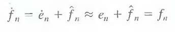
In order to accommodate the insertion of the quantization step, the error-free encoder of figure must be altered so that the predictions generated by the encoder and decoder are equivalent. As Fig.9 (a) shows, this is accomplished by placing the lossy encoder's predictor within a feedback loop, where its input, denoted f˙n, is generated as a function of past predictions and the corresponding quantized errors. That is,
![]()
This closed loop configuration prevents error buildup at the decoder's output. Note from Fig. 9
(b) that the output of the decoder also is given by the above Eqn.
Optimal predictors:
The optimal predictor used in most predictive coding applications minimizes the encoder's mean- square prediction error
![]()
subject to the constraint that
and
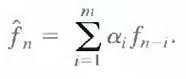
That is, the optimization criterion is chosen to minimize the mean-square prediction error, the quantization error is assumed to be negligible (e˙n ≈ en), and the prediction is constrained to a linear combination of m previous pixels.1 These restrictions are not essential, but they simplify the analysis considerably and, at the same time, decrease the computational complexity of the predictor. The resulting predictive coding approach is referred to as differential pulse code modulation (DPCM).