What is image compression. Explain about the redundancies in a digital image.

The term data compression refers to the process of reducing the amount of data required to represent a given quantity of information. A clear distinction must be made between data and information. They are not synonymous. In fact, data are the means by which information is conveyed. Various amounts of data may be used to represent the same amount of information. Such might be the case, for example, if a long-winded individual and someone who is short and to the point were to relate the same story. Here, the information of interest is the story; words are the data used to relate the information. If the two individuals use a different number of words to tell the same basic story, two different versions of the story are created, and at least one includes nonessential data. That is, it contains data (or words) that either provide no relevant information or simply restate that which is already known. It is thus said to contain data redundancy.

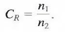
Data redundancy is a central issue in digital image compression. It is not an abstract concept but a mathematically quantifiable entity. If n₁ and n₂ denote the number of   information-carrying units in two data sets that represent the same information, the relative data redundancy R_D of the first data set (the one characterized by n₁) can be defined as

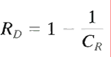
where C_R , commonly called the compression ratio, is

For the case n₂ = n₁, C_R = 1 and R_D = 0, indicating that (relative to the second data set) the first representation of the information contains no redundant data. When n₂ << n₁, C_R € ∞

nda

R_D€1,  implying  significant  compression  and  highly  redundant  data.  Finally,  when  n₂ >>  n₁

, C_R€  0  and  R_D €∞,  indicating  that  the  second  data  set  contains  much  more  data than the original representation. This, of course, is the normally undesirable case of data expansion. In general, C_R and R_D lie in the open intervals (0, ∞) and (- ∞, 1), respectively. A practical compression ratio, such as 10 (or 10:1), means that the first data set has 10 information carrying

units (say, bits) for every 1 unit in the second or compressed data set. The corresponding redundancy of 0.9 implies that 90% of the data in the first data set is redundant.

In digital image compression, three basic data redundancies can be identified and exploited: coding redundancy, interpixel redundancy, and psychovisual redundancy. Data compression is achieved when one or more of these redundancies are reduced or eliminated.

Coding Redundancy:

In this, we utilize formulation to show how the gray-level histogram of an image also   can provide a great deal of insight into the construction of codes to reduce the amount of data used to represent it.

Let us assume, once again, that a discrete random variable r_k in the interval [0, 1] represents the gray levels of an image and that each r_k occurs with probability p_r (r_k).

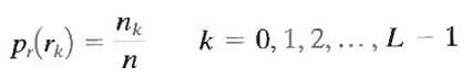
where L is the number of gray levels, n_k is the number of times that the kth gray level appears in the image, and n is the total number of pixels in the image. If the number of bits used to represent each value of r_k is l (r_k), then the average number of bits required to represent each pixel is

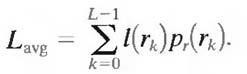
That is, the average length of the code words assigned to the various gray-level values is found by summing the product of the number of bits used to represent each gray level and the probability that the gray level occurs. Thus the total number of bits required to code an M X N image is MNL_avg.

Interpixel Redundancy:

Consider the images shown in Figs. 1.1(a) and (b). As Figs. 1.1(c) and (d) show, these images have virtually identical histograms. Note also that both histograms are trimodal, indicating the presence of three dominant ranges of gray-level values. Because the gray levels in these images are not equally probable, variable-length coding can be used to reduce the coding redundancy that would result from a straight or natural binary encoding of their pixels. The coding process, however, would not alter the level of correlation between the pixels within the images. In other words, the codes used to represent the gray levels of each image have nothing to do with the correlation between pixels. These correlations result from the structural or geometric relationships between the objects in the image.

Fig.1.1 Two images and their gray-level histograms and normalized autocorrelation coefficients along one line.

Figures 1.1(e) and (f) show the respective autocorrelation coefficients computed along one line of each image.

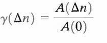
where

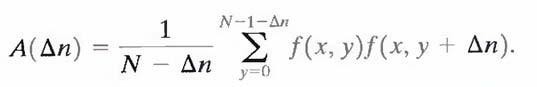
The scaling factor in Eq. above accounts for the varying number of sum terms that arise for each integer value of Δn. Of course, Δn must be strictly less than N, the number of pixels on a line. The variable x is the coordinate of the line used in the computation. Note the dramatic difference between the shape of the functions shown in Figs. 1.1(e) and (f). Their shapes can be qualitatively related to the structure in the images in Figs. 1.1(a) and (b).This relationship is particularly noticeable in Fig. 1.1 (f), where the high correlation between pixels separated by 45 and 90 samples can be directly related to the spacing between the vertically oriented matches of Fig. 1.1(b). In addition, the adjacent pixels of both images are highly correlated. When Δn is 1, γ is 0.9922 and 0.9928 for the images of Figs. 1.1 (a) and (b), respectively. These values are typical of most properly sampled television images.

These illustrations reflect another important form of data redundancy—one directly related to the interpixel correlations within an image. Because   the value of any given pixel can be reasonably predicted from the value of its neighbors, the information carried by individual pixels is relatively small. Much of the visual contribution of a single pixel to an image is redundant; it could have been guessed on the basis of the values of its neighbors. A variety of names, including spatial redundancy, geometric redundancy, and interframe redundancy, have been coined to refer to these interpixel dependencies. We use the term interpixel redundancy to encompass them all.

In order to reduce the interpixel redundancies in an image, the 2-D pixel array normally used for human viewing and interpretation must be transformed into a more efficient (but usually "nonvisual") format. For example, the differences between adjacent pixels can be used to represent an image. Transformations of this type (that is, those that remove interpixel redundancy) are referred to as mappings. They are called reversible mappings if the original image elements can be reconstructed from the transformed data set.

Psychovisual Redundancy:

The brightness of a region, as perceived by the eye, depends on factors other than simply   the light reflected by the region. For example, intensity variations (Mach bands) can be perceived in an area of constant intensity. Such phenomena result from the fact that the eye does not respond with equal sensitivity to all visual information. Certain information simply has less relative importance than other information in normal visual processing. This information is said to be psychovisually redundant. It can be eliminated without significantly impairing the quality of image perception.

That psychovisual redundancies exist should not come as a surprise, because human perception of the information in an image normally does not involve quantitative analysis of every pixel value in the image. In general, an observer searches for distinguishing features such as edges or textural regions and mentally combines them into recognizable groupings. The brain then correlates these groupings with prior knowledge in order to complete the image interpretation process. Psychovisual redundancy is fundamentally different from the redundancies discussed earlier. Unlike coding and interpixel redundancy, psychovisual redundancy is associated with real or quantifiable visual information. Its elimination is possible only because the information itself is not essential for normal visual processing. Since the elimination of psychovisually redundant data results in a loss of quantitative information, it is commonly referred to as quantization.

This terminology is consistent with normal usage of the word, which generally means the mapping of a broad range of input values to a limited number of output values. As it is an irreversible operation (visual information is lost), quantization results in lossy data compression.