Explain about the edge linking procedures.

The different methods for edge linking are as follows

• Local processing
• Global processing via the Hough Transform
• Global processing via graph-theoretic techniques.

(i)   Local Processing:

One of the simplest approaches for linking edge points is to analyze the characteristics of pixels in a small neighborhood (say, 3 X 3 or 5 X 5) about every point (x, y) in an image that has been labeled an edge point. All points that are similar according to a set of predefined criteria are linked, forming an edge of pixels that share those criteria.

The two principal properties used for establishing similarity of edge pixels in this kind of analysis are (1) the strength of the response of the gradient operator used to produce the edge

pixel; and (2) the direction of the gradient vector. The first property is given by the value of Af.

Thus an edge pixel with coordinates (x_o, y_o) in a predefined neighborhood of (x, y), is similar in magnitude to the pixel at (x, y) if

The direction (angle) of the gradient vector is given by Eq. An edge pixel at (x_o, y_o) in the predefined neighborhood of (x, y) has an angle similar to the pixel at (x, y) if

where A is a nonnegative angle threshold. The direction of the edge at (x, y) is perpendicular to the direction of the gradient vector at that point.

A point in the predefined neighborhood of (x, y) is linked to the pixel at (x, y) if both magnitude and direction criteria are satisfied. This process is repeated at every location in the image. A record must be kept of linked points as the center of the neighborhood is moved from pixel to pixel. A simple bookkeeping procedure is to assign a different gray level to each set of linked edge pixels.

(2)     Global processing via the Hough Transform:

In this process, points are linked by determining first if they lie on a curve of specified shape. We now consider global relationships between pixels. Given n points in an image, suppose that we want to find subsets of these points that lie on straight lines. One possible solution is to first find all lines determined by every pair of points and then find all subsets of points that are close to particular lines. The problem with this procedure is that it involves finding n(n - 1)/2 ~ n² lines and then performing (n)(n(n - l))/2 ~ n³ comparisons of every point to all lines. This approach is computationally prohibitive in all but the most trivial applications.

Hough [1962] proposed an alternative approach, commonly referred to as the Hough transform. Consider a point (x_i, y_i) and the general equation of a straight line in slope-intercept form, y_i = a.x_i + b. Infinitely many lines pass through (x_i, y_i) but they all satisfy the equation y_i = a.x_i + b for varying values of a and b. However, writing this equation as b = -a.x_i + y_i, and considering the ab-plane (also called parameter space) yields the equation of a single line for a fixed pair (x_i, y_i). Furthermore, a second point (x_j, y_j) also has a line in parameter space associated with it, and this line intersects the line associated with (x_i, y_i) at (a', b'), where a' is the slope and b' the intercept of the line containing both (x_i, y_i) and (x_j, y_j) in the xy-plane. In fact, all points contained on this line have lines in parameter space that intersect at (a', b'). Figure 3.1 illustrates these concepts.

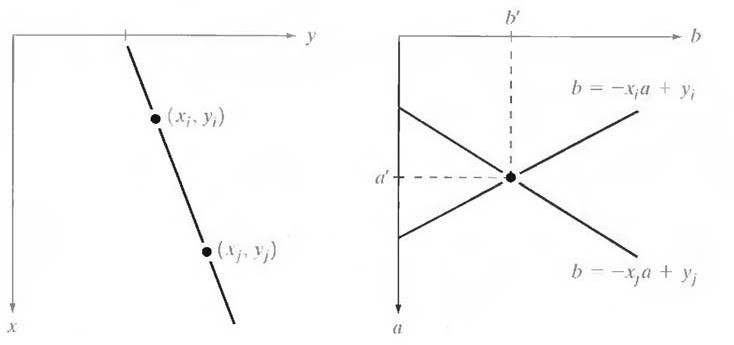
Fig.3.1 (a) xy-plane (b) Parameter space

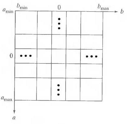
Fig.3.2 Subdivision of the parameter plane for use in the Hough transform

The computational attractiveness of the Hough transform arises from subdividing the parameter space into so-called accumulator cells, as illustrated in Fig. 3.2, where (a_max ,   a_min)   and (b_max , b_min), are the expected ranges of slope and intercept values. The cell at coordinates (i, j), with accumulator value A(i, j), corresponds to the square associated with parameter space coordinates (a_i , b_i).

Initially, these cells are set to zero. Then, for every point (x_k, y_k) in the image plane, we let the parameter a equal each of the allowed subdivision values on the fl-axis and solve for the corresponding b using the equation b = - x_k a + y_k .The resulting b’s are then rounded off to the nearest allowed value in the b-axis. If a choice of a_p results in solution b_q, we let A (p, q) = A (p,

1. q) + 1. At the end of this procedure, a value of Q in A (i, j) corresponds to Q points in the xy- plane lying on the line y = a_i x + b_j. The number of subdivisions in the ab-plane determines the accuracy of the co linearity of these points. Note that subdividing the a axis into K increments gives, for every point (x_k, y_k), K values of b corresponding to the K possible values of a. With n image points, this method involves nK Thus the procedure just discussed is linear in n, and the product nK does not approach the number of computations discussed at the beginning unless K approaches or exceeds n.

A problem with using the equation y = ax + b to represent a line is that the slope approaches infinity as the line approaches the vertical. One way around this difficulty   is to use the normal representation of a line:

x cosθ + y sinθ = ρ

Figure 3.3(a) illustrates the geometrical interpretation of the parameters used. The use of this representation in constructing a table of accumulators is identical to the method discussed for the slope-intercept representation. Instead of straight lines, however, the loci are sinusoidal curves in the ρθ -plane. As before, Q collinear points lying on a line x cosθ_j + y sinθ_j = ρ, yield   Q sinusoidal curves that intersect at (p_i, θ_j) in the parameter space. Incrementing θ and solving for the corresponding p gives Q entries in accumulator A (i, j) associated with the cell determined by (p_i, θ_j). Figure 3.3 (b) illustrates the subdivision of the parameter space.

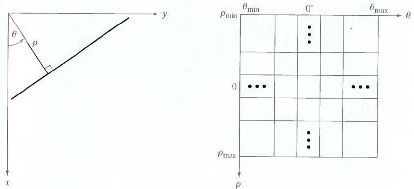
Fig.3.3 (a) Normal representation of a line (b) Subdivision of the ρθ-plane into cells

The range of angle θ is ±90°, measured with respect to the x-axis. Thus with reference to Fig. 3.3 (a), a horizontal line has θ = 0°, with ρ being equal to the positive x-intercept. Similarly, a vertical line has θ = 90°, with p being equal to the positive y-intercept, or θ = - 90°, with ρ being equal to the negative y-intercept.

(3)       Global processing via graph-theoretic techniques

In this process we have a global approach for edge detection and linking based on representing edge segments in the form of a graph and searching the graph for low-cost paths that correspond to significant edges. This representation provides a rugged approach that performs well in the presence of noise.

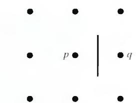
Fig.3.4 Edge clement between pixels p and q

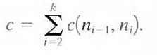
We begin the development with some basic definitions. A graph G = (N,U) is a finite, nonempty set of nodes N, together with a set U of unordered pairs of distinct elements of N. Each pair (n_i, n_j) of U is called an arc. A graph in which the arcs are directed is called a directed graph. If an arc is directed from node n_i to node n_j, then n_j is said to be a successor of the parent node n_i. The process of identifying the successors of a node is called expansion of the node. In each graph we define levels, such that level 0 consists of a single node, called the start or root node, and the nodes in the last level are called goal nodes. A cost c (n_i, n_j) can be associated with every arc (n_i, n_j). A sequence of nodes n₁, n₂... n_k, with each node n_i being a successor of node n_i-1 is called a path from n₁ to n_k. The cost of the entire path is

The following discussion is simplified if we define an edge element as the boundary between two pixels p and q, such that p and q are 4-neighbors, as Fig.3.4 illustrates. Edge elements are identified by the xy-coordinates of points p and q. In other words, the edge element in Fig. 3.4 is defined by the pairs (x_p, y_p) (x_q, y_q). Consistent with the definition an edge is a sequence of connected edge elements.

We can illustrate how the concepts just discussed apply to edge detection using the 3 X 3 image shown in Fig. 3.5 (a). The outer numbers are pixel

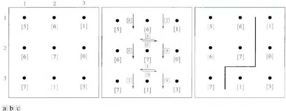
Fig.3.5 (a) A 3 X 3 image region, (b) Edge segments and their costs, (c) Edge corresponding to the lowest-cost path in the graph shown in Fig. 3.6

coordinates and the numbers in brackets represent gray-level values. Each edge element, defined by pixels p and q, has an associated cost, defined as

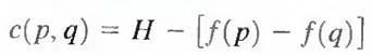
where H is the highest gray-level value in the image (7 in this case), and f(p) and f(q) are the gray- level values of p and q, respectively. By convention, the point p is on the right-hand side of the direction of travel along edge elements. For example, the edge segment (1, 2) (2, 2) is between points (1, 2) and (2, 2) in Fig. 3.5 (b). If the direction of travel is to the right, then p is the point with coordinates (2, 2) and q is point with coordinates (1, 2); therefore, c (p, q) = 7 - [7

- 6] = 6. This cost is shown in the box below the edge segment. If, on the other hand, we are traveling to the left between the same two points, then p is point (1, 2) and q is (2, 2). In this case the cost is 8, as shown above the edge segment in Fig. 3.5(b). To simplify the discussion, we assume that edges start in the top row and terminate in the last row, so that the first element of an edge can be only between points (1, 1), (1, 2) or (1, 2), (1, 3). Similarly, the last edge element has

to be between points (3, 1), (3, 2) or (3, 2), (3, 3). Keep in mind that p and q are 4-neighbors, as noted earlier. Figure 3.6 shows the graph for this problem. Each node (rectangle) in the graph corresponds to an edge element from Fig. 3.5. An arc exists between two nodes if the two corresponding edge elements taken in succession can be part of an edge.

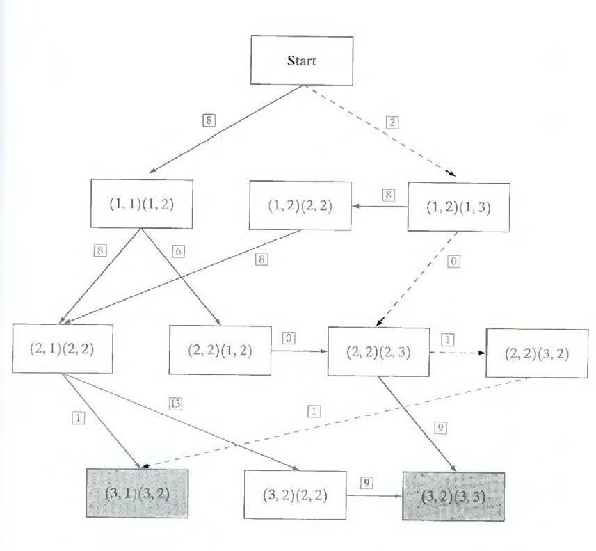
Fig. 3.6 Graph for the image in Fig.3.5 (a). The lowest-cost path is shown dashed.

As in Fig. 3.5 (b), the cost of each edge segment, is shown in a box on the side of the arc leading into the corresponding node. Goal nodes are shown shaded. The minimum cost path is shown dashed, and the edge corresponding to this path is shown in Fig. 3.5 (c).